The backpropagation method is an extension of the perceptron method for acyclic artificial neural networks. Acyclic artificial neural networks are defined in terms of the following:
functions f1, f2, f3, ..., fN
weight matrices W1, W2, W3, ..., WN
bias vectors b1, b2, b3, ..., bN
such that the result for an input vector i involves:
o0 = i
oj = (fj (aj1), fj (aj2), fj (aj3), ..., fj (ajN)) for j = 1, 2, 3, ..., N
aj = Wj oj -1 + bj for j = 1, 2, 3, ..., N
where oN is the result.
In the backpropagation method, each weight matrix and bias vector is updated for each input output vector pair (i, o) by subtracting a small fraction of the corresponding partial derivative of the error function Eo = (o - oN)2 / 2. The small fraction is referred to as the learning rate. For a derivation of the formulas to calculate these partial derivatives, click here.
Here is sample Python backpropagation method code:
#!/usr/bin/env python3
"""
Implements the backpropagation method.
Usage:
./backprop <data file> \
<data split> \
<number of hidden layers> \
<number of hidden layer functions> \
<number of categories> \
<learning rate> \
<number of epochs>
Data files must be space delimited with one input output pair per line.
Every hidden layer has the same number of functions.
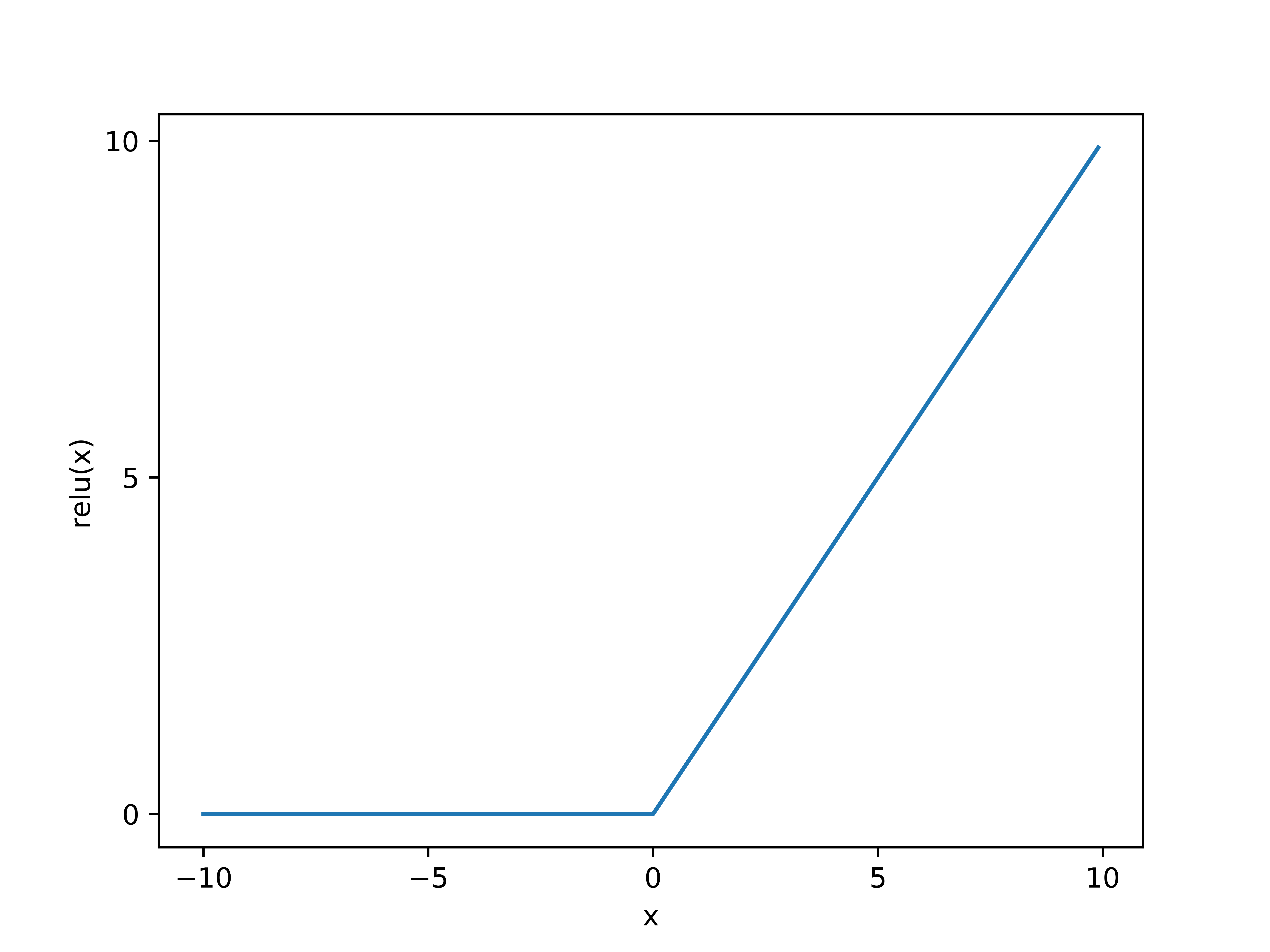
The hidden layer functions are rectified linear unit functions.
The outer layer functions are identity functions.
initialization steps:
The input output pairs are shuffled and the inputs mix max normalized.
The weights and biases are set to random values.
Requires NumPy.
"""
import numpy
import sys
def min_max(data):
"""
Finds the min max normalizations of data.
"""
return (data - numpy.min(data)) / (numpy.max(data) - numpy.min(data))
def init_data(data_file, data_split, n_cat):
"""
Creates the training and testing data.
"""
data = numpy.loadtxt(data_file)
numpy.random.shuffle(data)
data[:, :-1] = min_max(data[:, :-1])
outputs = numpy.identity(n_cat)[data[:, -1].astype("int")]
data = numpy.hstack((data[:, :-1], outputs))
data_split = int((data_split / 100) * data.shape[0])
return data[:data_split, :], data[data_split:, :]
def accuracy(data, weights, biases, n_cat):
"""
Calculates the accuracies of models.
"""
results = model(data[:, :-n_cat], weights, biases)
outputs = numpy.argmax(data[:, -n_cat:], 1)
return 100 * (results == outputs).astype(int).mean()
def model_(inputs, weights, biases, relu = True):
"""
model helper function
"""
results = numpy.matmul(weights, inputs.T).T + biases
if relu:
results = numpy.maximum(results, 0)
return results
def model(inputs, weights, biases):
"""
Finds the model results.
"""
results = model_(inputs, weights[0], biases[0])
for e in zip(weights[1:-1], biases[1:-1]):
results = model_(results, e[0], e[1])
results = model_(results, weights[-1], biases[-1], False)
results = numpy.argmax(results, 1)
return results
def adjust(weights, biases, input_, output, func_inps, func_outs, learn_rate):
"""
Adjusts the weights and biases.
"""
d_e_f_i = [func_outs[-1] - output]
d_e_w = [numpy.outer(d_e_f_i[-1], func_outs[-2])]
for i in reversed(range(len(weights) - 1)):
func_deriv = numpy.clip(numpy.sign(func_inps[i]), 0, 1)
vector = numpy.matmul(weights[i + 1].T, d_e_f_i[-1])
func_out = func_outs[i - 1] if i else input_
d_e_f_i.append(numpy.multiply(vector, func_deriv))
d_e_w.append(numpy.outer(d_e_f_i[-1], func_out))
for i, e in enumerate(reversed(list(zip(d_e_w, d_e_f_i)))):
weights[i] -= learn_rate * e[0]
biases[i] -= learn_rate * e[1]
def learn(train_data, n_hls, n_hl_funcs, n_cat, learn_rate, n_epochs):
"""
Learns the weights and biases from the training data.
"""
weights = [numpy.random.randn(n_hl_funcs, train_data.shape[1] - n_cat)]
for i in range(n_hls - 1):
weights.append(numpy.random.randn(n_hl_funcs, n_hl_funcs))
weights.append(numpy.random.randn(n_cat, n_hl_funcs))
weights = [e / numpy.sqrt(e.shape[0]) for e in weights]
biases = [numpy.random.randn(n_hl_funcs) for i in range(n_hls)]
biases.append(numpy.random.randn(n_cat))
biases = [e / numpy.sqrt(e.shape[0]) for e in biases]
for i in range(n_epochs):
for e in train_data:
input_ = e[:-n_cat]
func_inps = []
func_outs = []
for l in range(n_hls + 1):
input__ = func_outs[l - 1] if l else input_
func_inp = numpy.matmul(weights[l], input__)
func_inp += biases[l]
relu = numpy.maximum(func_inp, 0)
func_out = relu if l != n_hls else func_inp
func_inps.append(func_inp)
func_outs.append(func_out)
adjust(weights,
biases,
e[:-n_cat],
e[-n_cat:],
func_inps,
func_outs,
learn_rate)
return weights, biases
n_cat = int(sys.argv[5])
train_data, test_data = init_data(sys.argv[1], float(sys.argv[2]), n_cat)
weights, biases = learn(train_data,
int(sys.argv[3]),
int(sys.argv[4]),
n_cat,
float(sys.argv[6]),
int(sys.argv[7]))
print(f"weights and biases: {weights}, {biases}")
accuracy_ = accuracy(train_data, weights, biases, n_cat)
print(f"training data accuracy: {accuracy_:.2f}%")
accuracy_ = accuracy(test_data, weights, biases, n_cat)
print(f"testing data accuracy: {accuracy_:.2f}%")
Here are sample results for the MNIST dataset (Modified National Institute Of Standards And Technology dataset) available from many sources such as Kaggle:
./backprop MNIST_dataset 80 2 64 10 0.001 100
weights and biases: [array([[ 0.20884894, -0.02542065, -0.10987643, ..., -0.15665534,
-0.08775792, 0.0638999 ],
[-0.00592018, 0.18332229, -0.01387026, ..., 0.06527793,
0.13211286, 0.09518377],
...
0.00713001, -0.402518 , 0.21595368, 0.3279246 , -0.02778006,
0.01107208, 0.03471949, -0.27601775, -0.21284684, -0.1401997 ,
-0.20863759, -0.05693757, 0.09183485, -0.06464501]), array([-0.01450932, -0.00257944, -0.02661391, 0.026662 , -0.01042119,
-0.04099369, 0.66813539, 0.50147859, -0.08111961, -0.0198442 ])]
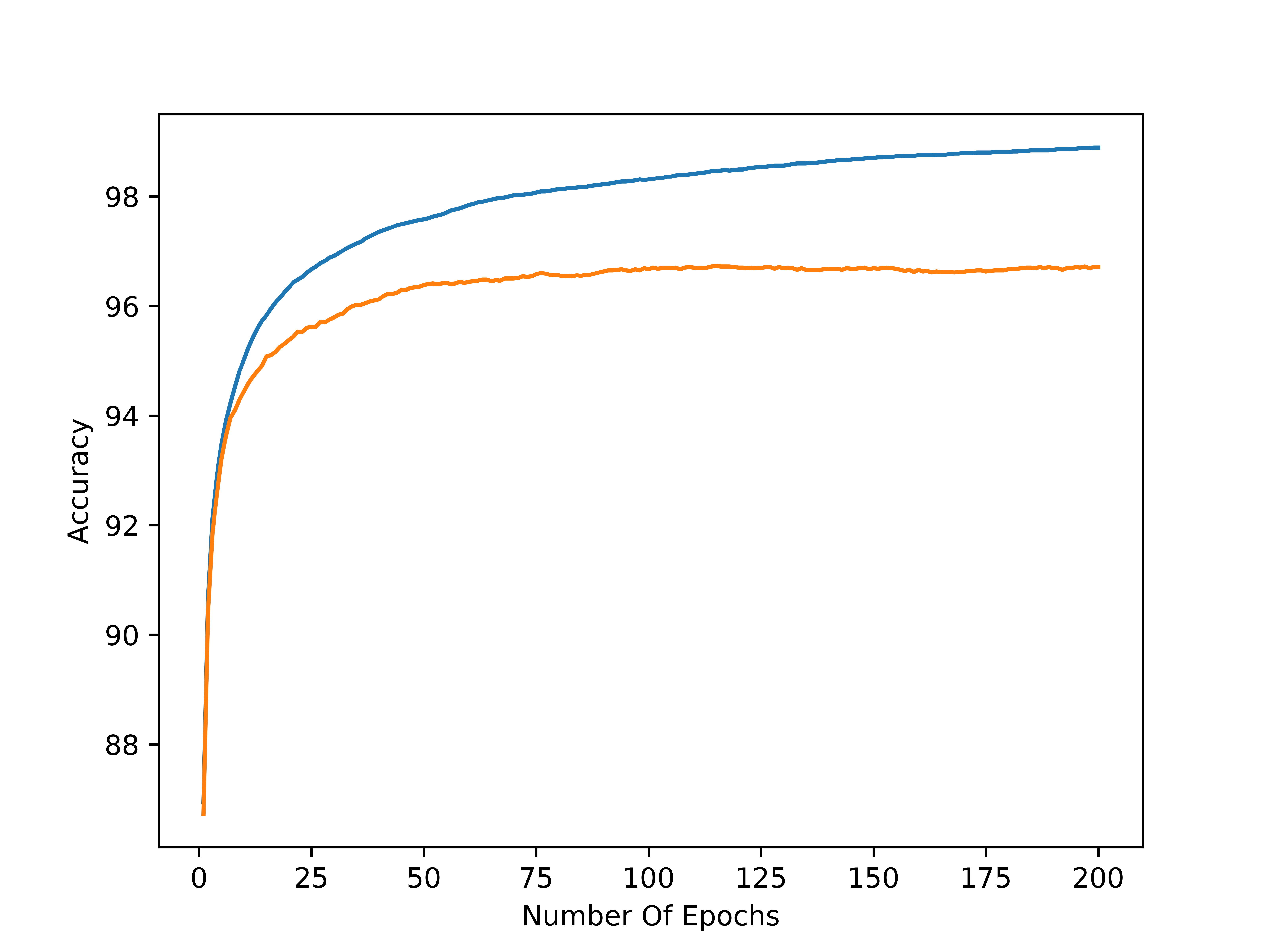
training data accuracy: 98.15%
testing data accuracy: 96.43%
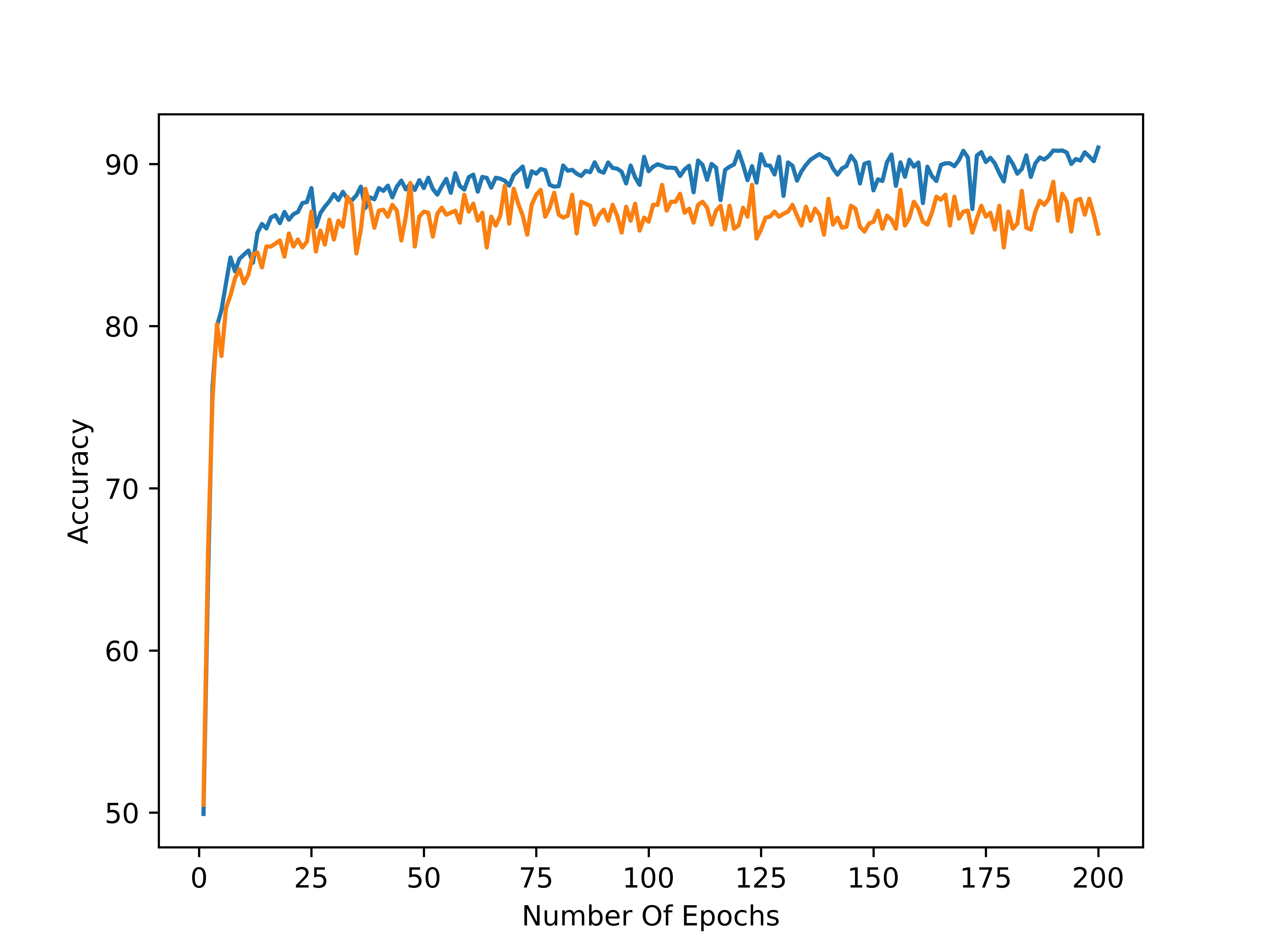
Here is a plot of the accuracy versus the number of epochs for a data split of 80 / 20, two hidden layers, 64 functions per hidden layer, 10 categories, and, a learning rate of 0.001. Blue denotes the training data accuracy and orange denotes the testing data accuracy: